Tutorial: Visualizing your rFon1D results
This document will walk you through the steps of how to visualize your rFon1D outputs from ortho_seqs using the rf1d-viz CLI command.
Note: rf1d-viz assumes that you have already run orthogonal_polynomial on the dataset. For a tutorial on how to run orthogonal_polynomial, view the tutorial here.
1. Requirements for rf1d-viz
The {trait_file_name}_regressions.npz file that is returned from orthogonal-polynomial.
The rf1d form of the alphabet input.
When you run orthogonal-polynomial, the CLI will output the following text towards the beginning:
rf1d form of alphabet input:
The line beneath that line is the rf1d form of the alphabet input.
The molecule type of the sequence (mostly DNA or protein).
What the phenotype values are representing.
2. rf1d-viz flags:
rf1d-viz will require you to input the following flags, many of which have counterparts in orthogonal-polynomial:
--filename
This will be the {trait_file_name}_regressions.npz file that is returned from orthogonal-polynomial.
--alphbt_input
This will be the rf1d form of the alphabet input.
--molecule
This is the molecule type.
--phenotype
This is the phenotype type. It will be used for labelling the graphs.
--out_dir
This is where you want the graphs stored. Note: the path must exist prior to running rf1d-viz.
--action
This is where you specify what kind of visualization you want. The current options are:
barplot - This will create a barplot of the rFon1D values, grouped by site and alphabet input. This is called automatically when you run orthogonal-polynomial.
density - This will create a density plot of the rFon1D values.
summary - Prints out the number of sites and dimensions, the alphabet input, the molecule, and calls sort (another rf1d-viz action that is explained in further detail below). This is called in orthogonal-polynomial automatically, and will not be saved.
heatmap - This will create a heatmap of the rFon1D values, grouped by site and alphabet input.
boxplot - This will create a boxplot of the rFon1D values, grouped by .
sort - This will print out the top 10 rFon1D values by magnitude, including the rFon1D value, the site, and the group it belongs to. This will not be saved to the out_dir.
ALL - This will produce a barplot, histogram, heatmap, and boxplot simultaneously.
Note: For now, you will need to close the first graph once it displays on your computer for the rest of the graphs to run.
3. Running rf1d-viz
Similarly to orthogonal-polyomial, you will run rf1d-viz in your CLI, first starting with the keyword ortho_seq, but now followed by rf1d-viz, instead of orthogonal-polynomial. The general format is
ortho_seq rf1d-viz filename --alphbt_input --molecule --phenotype --out_dir --action
where filename represents the –filename flag.
Guided example with the Sidhu dataset
The example uses the Sidhu dataset, which is the same as was used for the orthogonal-polynomial tutorial. Recall that the input for orthogonal-polynomial was:
ortho_seq orthogonal-polynomial ortho_seq_code/Sidhu/Sidhu.xlsx --molecule protein --poly_order first --out_dir docs/source/tutorial_outputs --alphbt_input SYG,R --min_pct 40 --pheno_name ELISA
The regression file that will be used for rf1d-viz will thus be called
Sidhu_regressions.npz
Using the CLI output, we obtain
rf1d form of alphabet input:
SYG,R,z,n
which reveals that the rf1d form of the alphabet input is SYG,R,z,n.
With these in mind, the CLI input for rf1d-viz for a barplot will be
ortho_seq rf1d-viz docs/source/tutorial_outputs/Sidhu_regressions.npz --alphbt_input SYG,R,z,n --molecule protein --phenotype ELISA --out_dir docs/source/tutorial_outputs --action barplot
This line of code will reproduce the graph that is automatically run, and looks like
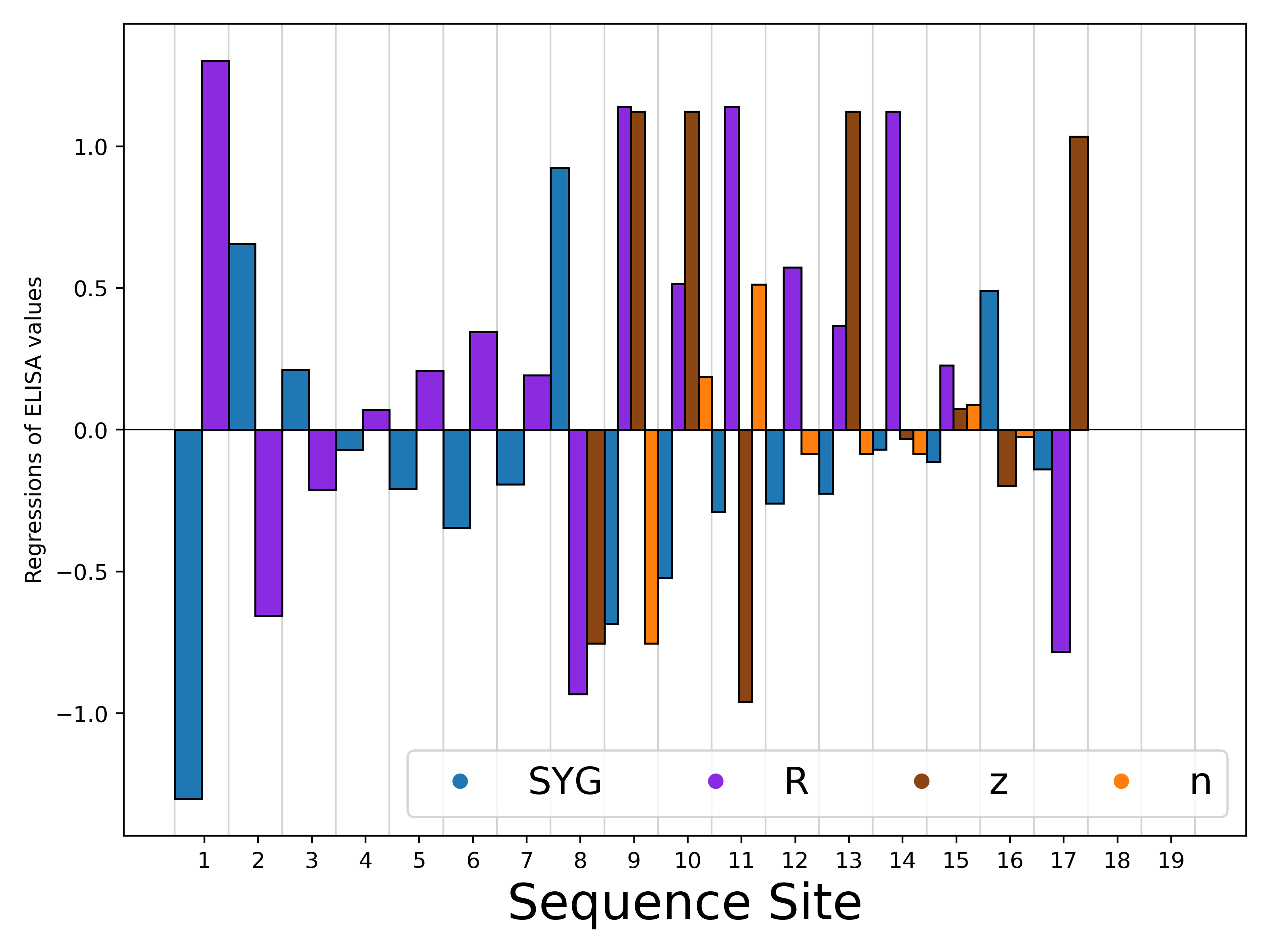
Notice how the y axis is labelled with the phenotype name specified
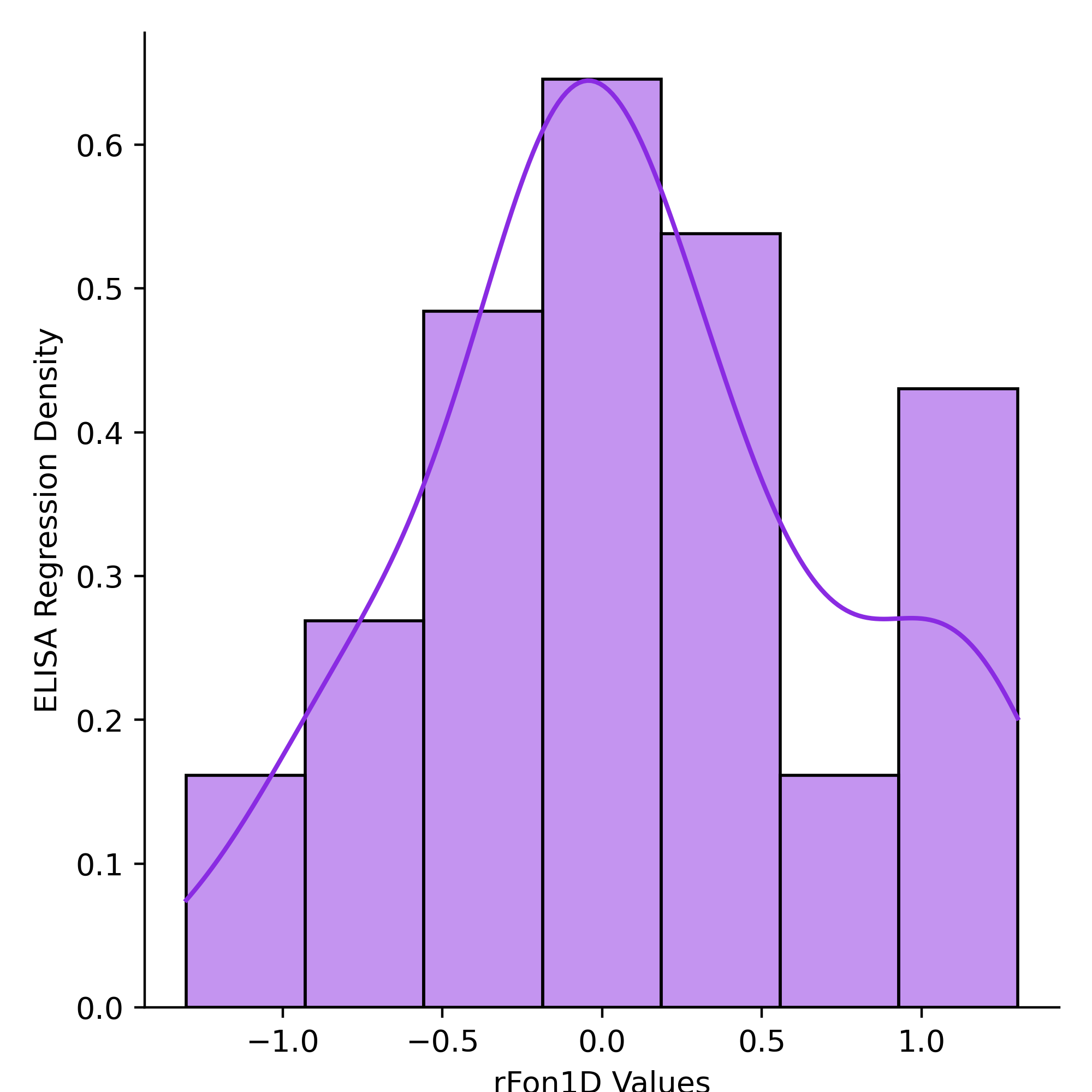
The CLI input for rf1d-viz for a density plot will be
ortho_seq rf1d-viz docs/source/tutorial_outputs/Sidhu_regressions.npz --alphbt_input SYG,R,z,n --molecule protein --phenotype ELISA --out_dir docs/source/tutorial_outputs --action density
The graph looks like
Run summary with
ortho_seq rf1d-viz docs/source/tutorial_outputs/Sidhu_regressions.npz --alphbt_input SYG,R,z,n --molecule protein --phenotype ELISA --out_dir docs/source/tutorial_outputs --action summary
The output will be
rf1d Object:

Number of sites: 19
Number of dimensions: 4
Alphabet input: ['SYG', 'R', 'z', 'n']
Molecule: protein

Phenotype represents ELISA values
Image output directory: docs/source/tutorial_outputs
Highest rFon1D magnitudes:
-1.3014       Site: 0         Key: SYG
1.3014        Site: 0         Key: R
1.1394        Site: 8         Key: R
1.1394        Site: 10                Key: R
1.1229        Site: 9         Key: z
1.1229        Site: 12                Key: z
1.1229        Site: 8         Key: z
1.1229        Site: 13                Key: R
1.0344        Site: 16                Key: z
-0.9606       Site: 10                Key: z
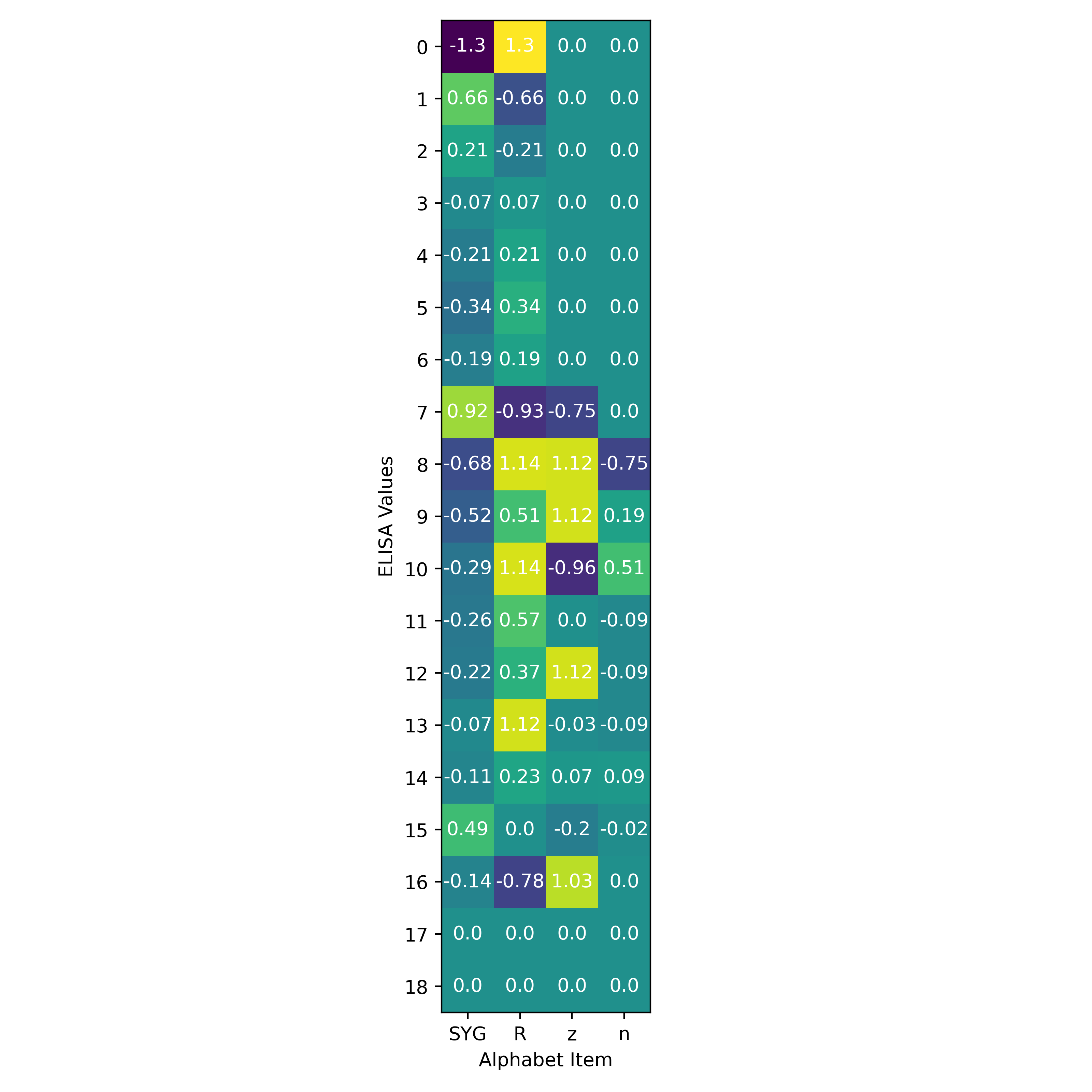
The CLI input for rf1d-viz for a heatmap will be
ortho_seq rf1d-viz docs/source/tutorial_outputs/Sidhu_regressions.npz --alphbt_input SYG,R,z,n --molecule protein --phenotype ELISA --out_dir docs/source/tutorial_outputs --action heatmap
The graph looks like
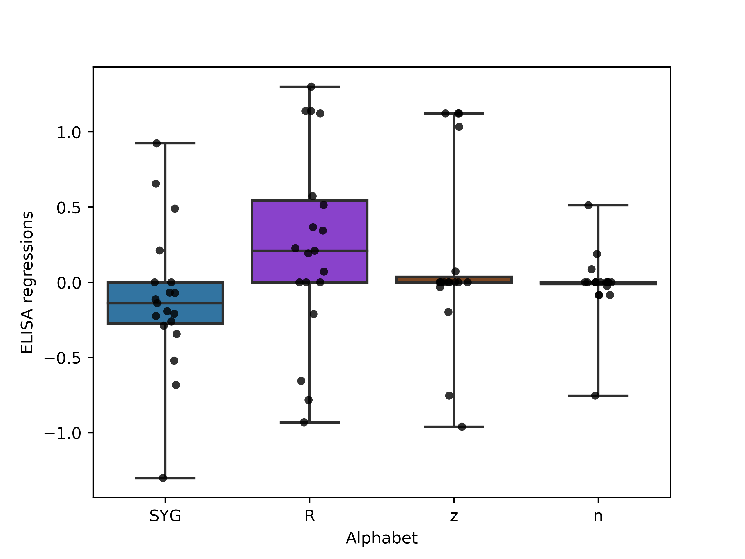
The CLI input for rf1d-viz for a boxplot will be
ortho_seq rf1d-viz docs/source/tutorial_outputs/Sidhu_regressions.npz --alphbt_input SYG,R,z,n --molecule protein --phenotype ELISA --out_dir docs/source/tutorial_outputs --action boxplot
The graph looks like
Lastly, this is the input for sort:
ortho_seq rf1d-viz docs/source/tutorial_outputs/Sidhu_regressions.npz --alphbt_input SYG,R,z,n --molecule protein --phenotype ELISA --out_dir docs/source/tutorial_outputs --action sort
The output will be
-1.3014       Site: 0         Key: SYG
1.3014        Site: 0         Key: R
1.1394        Site: 8         Key: R
1.1394        Site: 10                Key: R
1.1229        Site: 9         Key: z
1.1229        Site: 12                Key: z
1.1229        Site: 8         Key: z
1.1229        Site: 13                Key: R
1.0344        Site: 16                Key: z
-0.9606       Site: 10                Key: z
As you can see, this prints out the second half of the summary output, since summary calls sort.