Background & Quickstart
ortho_seqs
Ortho_seqs is a command line to convert sequence data (DNA/protein) to tensor-valued orthogonal polynomials and project phenotypes onto the polynomial space. We do this by first converting the sequence information into 4-dimensional (for DNA) or 20-dimensional (for amino acids) vectors. The method can also be used for padded sequences to deal with unequal sequence lengths. Find out more about the approach in this paper Analyzing genomic data using tensor-based orthogonal polynomials with application to synthetic RNAs. The paper gives an example of this method as applied to a case of synthetic RNA from a previously published dataset. Another manuscript detailing the use of this method to understand binding affinities of transcription factors (TFs) is currently in progress.
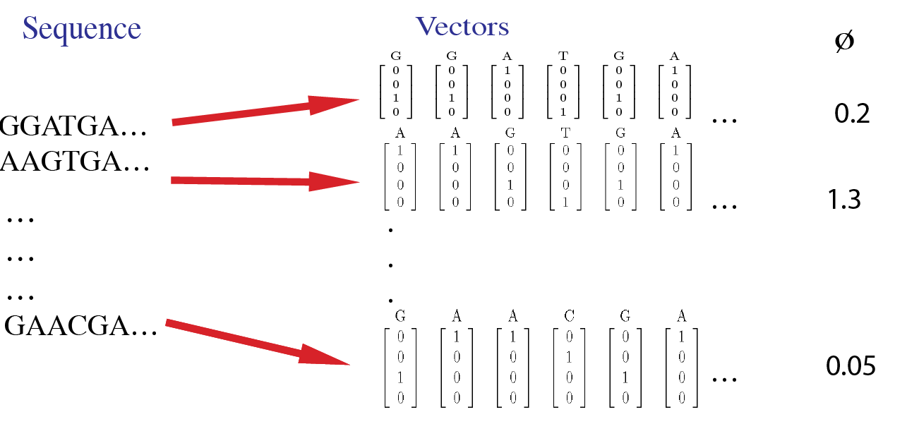
For example, the sample data inputs for this tool are shown in this image. Here, each site in a sequence is first converted to a 4-dimensional vector. The input data includes phenotype values for each sequence.
Usage
First, install an environment with dependencies for this package:
conda create -n ortho_seqs pip
pip install -r requirements.txt
conda activate ortho_seq
or
conda env create -f conda_environment.yml
conda activate ortho_seq
Then, install the package:
python setup.py install
Gather the input file(s) needed.
There are three main ways to submit your sequence and phenotype files to ortho_seqs. The first method is to submit them separately, in their own .txt files. Recently, however, an update was added that allows you to submit them both in the same file. For this to apply: 1) The file must be either a .xlsx or a .csv file. 2) The sequences must be in the first column, and the phenotypes must be in the second column. 3) The columns must not have header names.
If you use a single file for the sequence and phenotype, you would submit the file path where you would submit the sequence file path, and leave the –pheno_file flag blank (ortho_seqs will set that flag to None).
The phenotypes must be real numbers.
Then, to run the commandline tool:
To start with a test example, you can run the sample command below:
ortho_seq orthogonal-polynomial ./ortho_seq_code/tests/data/nucleotide/first_order/test_seqs_2sites_dna.txt --molecule DNA --pheno_file ./ortho_seq_code/tests/data/nucleotide/first_order/trait_test_seqs_2sites_dna.txt --poly_order second --out_dir ../results_ortho_seq_testing/DNA_2sites_test_run/
The above sample command line is building the tensor-valued orthogonal polynomial space based on the sequence data which consists of 12 sequences, each with two sites. Since these are DNA sequences, the vectors are 4-dimensional. These used to be flags for sites, dimensions, and population size, but new functionality will automatically calculate these. Corresponding to each sequence is a phenotype value (a real number) as given in the phenotype file. For DNA, the tool can run first and second order analyses currently. We’ll implement third order in a future version. For amino acids, the current version supports first order analysis and we hope to expand this in the future.
Amino acids/nucleotides that do not appear in any sequence will be removed from the alphabet when the letters are being converted to first order vectors. For example, if the residue ‘R’ (Arginine) never occurs in the sequence dataset, the first order vectors will now have 19 dimensions (instead of 20) and 20 dimensions (instead of 21) if the sequences are padded with ‘n’. This is done to greatly reduce runtime for larger sequence datasets and for longer sequences. When the program will run, it will return this sentence:
Will be computing p sequences with s sites, and each vector will be d-dimensional.
Where p represents the population size (number of rows in sequence file), s represents the number of sites, and d represents the number of amino acids/nucleotides detected in the sequence file (adds on 1 for lowercase n’s). For the above example, the program will return
Will be computing 12 sequences with 2 sites, and each vector will be 4-dimensional.
Along with regressions on each site independent of one another and onto two sites at a time, the above command also computes Fest which is the phenotype estimated by the regressions. This shows that the mathematical calculations are done correctly as we now have an equation that accurately captures our initial data points. This only works here for sequences with 2 sites. If we had more sites, we’d need to do higher order calculations in order to capture all our combinations. Therefore, when running the tool with more sites, as will probably be the case for most users, even just going up to second order gives us useful information about our system. First order tells us the importance of each site (independent of any correlations it might have with another site) and second order tells the importance of pairs of nucleotides independent of other pairs. Please take a look at the paper linked above to learn more about this method.
Flags & Functionality
--pheno_file
Input a file with phenotype values corresponding to each sequence in the sequence file. If you have a .xlsx or .csv file, do NOT use this flag (more details above in the Gather the Input Files Needed section).
   --molecule

Currently, you can provide DNA or protein sequences. Here, you can also provide sequences of unequal lengths, where sequences will be padded with lowercase 'n's until it has reached the length of the longest sequence.
–poly_order
The order of the polynomials that will be constructed. Currently, one can do first and second order for DNA and first order for protein.
–out_dir
Directory where results can be stored.
–precomputed
Let's say you have a case where you have the same set of sequences but two different corresponding sets of phenotypes. You can build your sequence space and then project the first set of phenotypes onto this space. Then, if you wish to see how the other set of phenotypes maps onto the same sequence space, you can use this flag so that you're not wasting time and memory to recompute the space. When doing this, be sure to add your results from the first run to the **out_dir** when rerunning the command with the **precomputed** flag.
–alphbt_input
Used to group amino acids/nucleotides together, or specify certain amino acids/nucleotides. If you don't want to group anything, don't include this flag when running *ortho_seqs*. For example, putting *ASGR* will tell the program to have 6 dimensions: one for each amino acid specified, and one for *z*, where every unspecified amino acid will be converted to *z*, and one for *n* (whenever sequences have unequal lengths, *ortho_seqs* will pad the shorter sequences with *n*). You can also comma-separate amino acids/nucleotides to group them. For example, putting *AS,GR* will make the vectors 4-dimensional, one for *AS*, one for *GR*, one for every other amino acid, and one for *n*.

There are also built-in groups:

**protein_pnp** will group by polar and non-polar amino acids, every other amino acid, and *n*.

**essential** groups by essential and non-essential amino acids, every other amino acid, and *n*. \
Group 1: Essential - ILVFWHKTM \
Group 2: Non-Essential - Everything else \
Group 3: n \
(Source: https://www.ncbi.nlm.nih.gov/books/NBK557845/)

**alberts** groups by categories set by Alberts. \
Group 1: Basic - KRH \
Group 2: Acidic - DE \
Group 3: AVLIPFMWGC \
Group 4: Everything else \
Group 5: n \
(Source: https://www.ncbi.nlm.nih.gov/books/NBK21054/)

**sigma** groups by categories set by Sigma. \
Group 1: Aliphatic - AILMV \
Group 2: Aromatic - FYV \
Group 3: Polar Neutral - NQCST \
Group 4: Acidic - KRH \
Group 5: Basic - DE \
Group 6: Other - G \
Group 7: Other - P \
Group 8: n \
(Source: https://www.sigmaaldrich.com/US/en/technical-documents/technical-article/protein-biology/protein-structural-analysis/amino-acid-reference-chart)

**hbond** groups by strength of hydrogen bond attractions. \
Group 1: Can Make Hydrogen Bonds - NQSTDERKYHW \
Group 2: Can Not Make Hydrogen Bonds - Everything else \
Group 3: n \
The first group is able to make hydrogen bonds, whereas the second group is not.

**hydrophobicity** groups by hydrophobicity. \
Group 1: Very Hydrophobic - LIFWVM \
Group 2: Hydrophobic - CYA \
Group 3: Neutral - TEGSQD \
Group 4: Hydrophilic - Everything else \
Group 4: n \
The first group is very hydrophobic, the second group is slightly hydrophobic, the third group is neutral, and the last group is hydrophilic.
–min_pct
When ortho_seqs is run, a .csv file of covariances will be saved in the specified path. This matrix of covariances is one of the main results of the program (as shown in {sequence_file_name}.npz output below). The csv file will contain the covariance of each nucleotide at each site with another nucleotide at another site (or amino acids at each site).
Suppose there are 5 covariance values of 2, 1, 0, 0, -1. For the percentiles, all unique *magnitudes* will be considered when assigning covariances, which will be 2, 1, and 0. 0 will be the 0th percentile (therefore, assigning 0 to the *--min_pct* flag will return every covariance), 1 (and -1) will be 33.33..., and 2 will be 66.66... Specifying 50 as *--min_pct* will only return the row with the covariance of 2, since only 66.6...>50.
The min_pct flag is short for minimum percentile, which will remove any covariances
from the .csv file that are below the given percentile. The default value is 75.
–pheno_name
Let's say you know that your phenotype values represent IC50 values. You could then add *--pheno_name IC50* as a flag, and on the rFon1D plot that is automatically generated, the y-axis label will include IC50. Default is **None**.

# Results & Outputs

The tool will provide updates as the run is progressing regarding which parts of the calculations are done being computed. For example, when the mean is computed, it'll say "computed mean". All the different elements that it is computing are different parts of building the multivariate tensor-valued orthogonal polynomial space based on the sequence information. To get a general idea of what the calculations mean, please refer to the supplementary methods in the paper linked above.
The program will save outputs in [npz format](https://numpy.org/doc/stable/reference/generated/numpy.savez.html). See below for what is stored.
{sequence_file_name}.npz
This will store the calculations that went into constructing the polynomial space. This also includes information about the statics of our sequence space, such as mean, variance and a matrix of covariances. See figures 4 and for ideas on how mean and the matrix of covariances can be visualized. All of these calculations go into building the orthogonal polynomial space based on sequence information and at this point of the program, we have not connected the phenotype (the functional variable) with the sequence information.
{sequence_file_name}_covs_with_F.npz
This will store the covariance of the phenotype (or trait) with the polynomials. This is when we start connecting the phenotype with the sequence space.
{trait_file_name}_Fm.npz
This contains the mean trait value. This is a scalar.
{trait_file_name}_regressions.npz
This set of files contains the main results which includes the following:
1. **rFon1D**: This is the regression of the trait onto the first order conditional polynomial orthogonalized within. This tells us the regression of the phenotype onto each site and onto each nucleotide (or amino acid) at that site independent of any correlations that site might have with other sites. For the case of nucleotides, this can be visualized as bar plots as shown in Figure 6 in the paper linked above.
2. **rFon2D**: This gives 4 matrices which give the regression of the pheonotype onto (site1)x(site1), (site 1)x(site 2), (site 2)x(site 1) and (site 2)x(site 2), in that order. The second matrix here is the important one and it is the same as rFon12. See description of rFon12.
3. **rFon12**: This is the regression of the trait onto *pairs* of sites for given nucleotides at each site. These are regressions on (site 1)x(site 2) independent of first order associations. Since we're looking at 2 sites at a time and there's a possibility of having 4 nucleotides at each site (for the case of DNA), we can visualize this via a 4x4 matrix as shown in Figure 8 in the paper linked above.
# The rf1d class
The newest update to *ortho_seqs* involves adding a new class of objects, called *rf1d* (short for rFon1D). To declare an *rf1d* object, you must supply a numpy ndarray of the rFon1D values (supplied via the regressions.npz file that is output when *ortho_seqs* is run), along with the alphabet input, and the molecule type.
Once you have done this, you can explore the rFon1D values, and see if there are any trends. You can:
1. Print out a summary of the object using .summary()
2. Make a bar plot (just like the rFon1D bar plot automatically generated) using .plot_bar()
3. Print out the extreme rFon1D values using .sort()
4. Remove any insignificant, but nonzero, rFon1D values using the .trim() function (**NOTE:** this will change the ndarray in the rf1d object, and to recover old data, you must reinstatiate an rf1d object)
5. Make a histogram of rFon1D values using .plot_hist()
# To run the GUI (currently in development)
A GUI version of the CLI is being actively developed in order to make it easier for users to utilize the tool. The GUI allows the user to upload the sequence and phenotype files via an upload button, specify the molecule, the polynomial order they wish to run, and whether the sequence space was already computed or not (via the precomputed button). The GUI is in its primitive form and will include further updates resembling the cli in future versions.

covhist{trait_file_name}.png
This is a histogram of all non-zero covariances. Its bin width is 0.5.
cov_dataframe{trait_file_name}.csv
This file is a csv file of covariances between every item at every site. This includes the item ID and site for both items in the pair used to calculate the covariance, the covariance value, the covariance magnitude, and an ID for the pair (s1-g2,s3-g4 represents the pairing of an element from the first group in the alphabet at the second site, and an element from the third group at the fourth site).
rFon1Dgraph{trait_file_name}.png ``` This is a bar plot of all nonzero rFon1D values of every item at every site.
Support
If you have specific or general questions, feel free to open an issue and we’ll do our best to address them. If you have any comments, suggestions or would like to chat about this method or similar ideas, feel free to reach out via email at saba.nafees314@gmail.com.
Roadmap
We hope to implement third order analysis for DNA in the near future. For amino acids, we hope to implement second order analysis. We’ll add visualization ideas soon but if you have any thoughts on this, please feel free to reach out.
Contribution
We hope to make the tool run faster as with higher dimenions and higher order analysis of longer sequence data, we can run into memory and time issues. Any thoughts on this or visualization are welcome.